Intro to dplyr tools

Quick overview

What do all these commands do?

This post was originally intended as a gentle introduction to the dplyr verbs for an undergraduate class on presidential elections. The text of this tutorial is taken largely from An Introduction to Statistical and Data Sciences via R.

The pipe (%>%)

Before we introduce the five main verbs, we first introduce the pipe operator (%>%). The pipe operator allows us to chain together data wrangling functions. The pipe operator can be read as “ then”. The (%>%) operator allows us to go from one step to the next easily so we can, for example:

• filter our data frame to only focus on a few rows then
• group_by another variable to create groups then
• summarize this grouped data to calculate the mean for each level of the group.

Five Main Verbs - The 5MV

The five most commonly used functions that help wrangle and summarize data. A description of these verbs follows, with each subsection devoted to an example of that verb, or a combination of a few verbs, in action.

This is a test

• filter: Pick rows based on conditions about their values
• summarise: Create summary measures of variables either over the entire data frame or over groups of observations on variables using group_by
• mutate: Create a new variable in the data frame by mutating existing ones
• arrange: Arrange/sort the rows based on one or more variables

All of the 5MVs follow the same syntax, with the argument before the pipe %>% being the name of the data frame, then the name of the verb, followed with other arguments specifying which criteria you’d like the verb to work with in parentheses.

Filter observations using filter

• The filter function here works much like the “Filter” option in Microsoft Excel; it allows you to specify criteria about values of a variable in your dataset and then chooses only those rows that match that criteria.

Example 1: Using words

• I want to view all of the rows (counties in this case) that have the state_name == Michigan. (All the counties in Michigan)

electiondta %>% 
  filter(state_name == "michigan")

The ordering of the commands:

• Take the data frame electiondta then
• filter the data frame so that only those where the state_name equals “Michigan” are included.
• The double equal sign == for testing for equality, and not=. You are almost guaranteed to make the mistake at least once of only including one equals sign

Example 2: Using numbers

• I want to view all of the rows (counties) that cast more than 100,000 total votes in 2012

electiondta %>% 
   filter(total_2012 > 100000)

The ordering of the commands:

• Take the data frame electiondta then
• filter the data frame so that only those where the total_2012 is greater than 100000 are included.

Other ways to filter

You can combine multiple criteria together using operators that make comparisons:

| corresponds to “or”	>= corresponds to “greater than or equal to”
& corresponds to “and”	<= corresponds to “less than or equal to”
> corresponds to “greater than”	!=corresponds to “not equal to”
< corresponds to “less than”

Summarise variables using summarize

The next common task when working with data is to be able to summarize data: take a large number of values and summarize then with a single value. While this may seem like a very abstract idea, something has simple as the sum, the smallest value, and the largest values are all summaries of a large number of values.

Example 1:

We can calculate the and mean and minimum, and maximum of the total number of votes for the democratic candidate in 2012 in one step using the summarize:

# A tibble: 1 x 3
    mean   min     max
   <dbl> <dbl>   <dbl>
1 20017.     5 1672164

What did that just do?

• Take the data frame electiondta then
• summarise the data frame so that so that we get the mean (or average) of the variable dem2012, the minimum value of dem2012 and the maximum value of 2012.

Other ways to use summarise

• IRQ(): Interquartile range
• sum(): the sum (or total)
• n(): a count of the number of rows/observations in each group. This will be really useful when you use group_by

Group rows using group_by

It’s often more useful to summarize a variable based on the groupings of another variable.

Example 1

Let’s say, we are interested in the mean of total votes cast in 2016 and total votes cast in 2012 but grouped by state. To be more specific: we want the mean and median votes cast in 2016

1. split by State
2. sliced by State
3. aggregated by State
4. collapsed over State

# A tibble: 50 x 3
   state_name           mean_20165 mean_2012
 * <chr>                     <dbl>     <dbl>
 1 alabama                  31017.    14562 
 2 arizona                 137521.    35775 
 3 arkansas                 14782.     6919 
 4 california              166068.    52330.
 5 colorado                 40065.     6658.
 6 connecticut             202943.   103224.
 7 delaware                147178.    93215 
 8 district of columbia    280272    243348 
 9 florida                 139521.    65958 
10 georgia                  25343.     9205 
# … with 40 more rows

Create new variables/change old variables using mutate

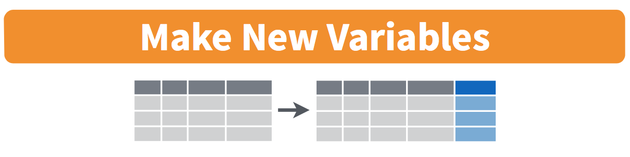
When looking at the electiondta dataset, there are some variables that were created using other variables in the dataset. For instance, the variable pct_dem_2012 refers to the percentage vote the Democratic candidate got in 2012. This variable was created by doing the following:

1. taking dem_2012 and dividing it by total_2012 to get a proportion.
2. Then, multiplying it by 100 to convert it to percentage points.

We will create this variable again using the mutate function.

Example 1: Creating pct_dem_2012

# A tibble: 3,122 x 4
   state_name county_name      pct_dem_2012_copy pct_dem_2012
   <chr>      <chr>                        <dbl>        <dbl>
 1 utah       Utah County                   9.79         9.79
 2 utah       Cache County                 14.6         14.6 
 3 idaho      Madison County                5.77         5.77
 4 utah       Davis County                 18.1         18.1 
 5 utah       Morgan County                 8.83         8.83
 6 utah       Box Elder County             10.1         10.1 
 7 utah       Salt Lake County             38.8         38.8 
 8 utah       Wasatch County               23.0         23.0 
 9 utah       Weber County                 25.8         25.8 
10 utah       Tooele County                23.1         23.1 
# … with 3,112 more rows

What did we just do?

1. Take the data frame electiondta then
2. create a variable that we are calling pct_dem_2012_copy that is equal to (dem_2012/total_2012)*100 then
3. To make the results easily viewable we are selecting state_name, county_name, pct_dem_2012_copy, and the original variable pct_dem_2012 for comparison

Using the original variable as a check, we can see that our pct_dem_2012_copy, the only difference being that our measure extends by a few decimal places.

Reorder the data frame using arrange

One of the most common things people working with data would like to do is sort the data frames by a specific variable in a column. Have you ever been asked to calculate a median by hand? This requires you to put the data in order from smallest to highest in value. The dplyr package has a function called arrange that we will use to sort/reorder our data according to the values of the specified variable. This is often used after we have used the group_by and summarize functions as we will see.

Let’s suppose we are interested in determining the states with the largest numbers of counties that were won by Trump.

# A tibble: 48 x 3
# Groups:   state_name [48]
   state_name  trump_county trump_counties
   <chr>       <chr>                 <int>
 1 alabama     Trump Won                54
 2 arizona     Trump Won                11
 3 arkansas    Trump Won                67
 4 california  Trump Won                26
 5 colorado    Trump Won                41
 6 connecticut Trump Won                 2
 7 delaware    Trump Won                 2
 8 florida     Trump Won                59
 9 georgia     Trump Won               128
10 idaho       Trump Won                42
# … with 38 more rows

OK great! But it looks like these are all out of order. So, we can just use arrange() to get them sorted. arrange() will automatically sort in ascending order (smallest to largest or A to Z) unless you tell it differently. Since we do, we need to let it know we want it sorted in descending order to get the largest numbers on the top.

# A tibble: 48 x 3
# Groups:   state_name [48]
   state_name trump_county trump_counties
   <chr>      <chr>                 <int>
 1 texas      Trump Won               228
 2 georgia    Trump Won               128
 3 kentucky   Trump Won               118
 4 missouri   Trump Won               111
 5 kansas     Trump Won               103
 6 iowa       Trump Won                93
 7 tennessee  Trump Won                92
 8 illinois   Trump Won                91
 9 nebraska   Trump Won                91
10 indiana    Trump Won                88
# … with 38 more rows

What did that code just do?

electiondta %>%
  filter(trump_county == "Trump Won") %>%
  group_by(state_name, trump_county) %>%
  summarise(trump_counties = n()) %>%
  arrange(desc(trump_counties))

1. Take the data frame electiondta then
2. Filter the data, since we are only interested in the counties that Trump won (using trump_county) then
3. Group the data by state (using state_name) and whether or not Trump won (using trump_county) then
4. Summarise the data to get a count of the number of counties Trump won (using n()) then
5. Arrange the data in descending order of trump_counties so we can see which states are the largest.